In the paper, orbital dynamics, regular or chaotic, of globular clusters (GCs) in the central region of the Galaxy, which is subject to the greatest influence of the rotating bar, has been studied. Such methods for determining chaos as Poincar´e sections and spectral methods have been compared. The relationship between the Poincar´e sections and the spectral characteristics of the orbits has been estimated. The sample includes 45 globular clusters in the central region of the Galaxy with a radius of 3.5 kpc. To form the 6D-phase space required for integrating the orbits, the most accurate astrometric data to date from the Gaia satellite, as well as new refined average distances, have been used. The following, most realistic, bar parameters have been adopted: mass 1010M⊙, length of the major semi-axis of the bar model in the form of a triaxial ellipsoid is 5 kpc, angle of rotation of the bar axis is 25o, rotation velocity is 40 km s−1 kpc −1. The result of the study is that a 100% correlation between the classification by Poincar´e sections and the spectral characteristics of the orbits has been established. Consequently, the classification by Poincar´e sections can be replaced by a more visual analysis of the amplitude spectra of the orbits. Thus, two lists of GCs: with regular and chaotic dynamics have been compiled. The GCs with varying degrees of orbital chaos have separately been distinguish.

This study is essentially a continuation of [1–3] devoted to the study of the orbital dy- namics (regular or chaotic) of globular clusters in the central region of the Galaxy. As in previous studies, the sample includes 45 globular clusters in the central region of the Galaxy with a radius of 3.5 kpc. To form the 6D-phase space required for orbit integra- tion, the most accurate astrometric data to date from the Gaia satellite [4], as well as new refined mean distances [5], were used. The following most realistic parameters of the bar that are known from the literature [6, 7] are adopted: the mass is 1010M⊙, the length of the major semi-axis is 5 kpc, the rotation angle of the bar axis is 25o, and the rotation speed is 40 km s−1 kpc −1. Since GCs in the central region of the Galaxy are subject to the greatest influence from the elongated rotating bar, the question of the nature of the orbital motion of GCs (regular or chaotic) is of great interest. For example, in [8], it is shown that the main share of chaotic orbits must be precisely in the bar region. This study is aimed at establishing the connection between Poincar´e sections and spec- tral characteristics of orbits as functions of time. Spectral methods include, in particular, the frequency method [9–13]. The authors of these studies showed that it is possible to measure the stochasticity of the orbit based on the shift of fundamental frequencies deter- mined over two consecutive time intervals. Another method of this class is our recently proposed method [3] based on calculating the orbital power spectrum as a function of time and calculating the entropy of the power spectrum as a measure of orbital chaos. The paper is structured as follows. In the first section, the accepted potential models: the axisymmetric potential and the non-axisymmetric potential including a bar is briefly described. In the second section, links to the used astrometric data, as well as the method for forming the GC sample, are provided. In the third section, the methods used to esti- mate the regularity/chaotic nature of motion: the Poincar´e section method, the frequency method, and the spectral methods we proposed are described. In the fourth section, the obtained results are analyzed and a connection between the Poincar´e cross sections and the spectral characteristics of the orbits are established. The main results of the study are formulated in the Conclusions section.

1galactic Potential Model

1.1 Axisymmetric Potential

The axisymmetric gravitational potential of the Galaxy traditionally used by us (see, for example, [2]) for integrating the orbits of GCs is represented as the sum of three components: the central spherical bulge Φb(r(R, Z)), disk Φd(r(R, Z)), and a massive spherical dark matter halo Φh(r(R, Z)):

Φ(R, Z) = Φb(r(R, Z)) + Φd(r(R, Z)) + Φh(r(R, Z)).             (1)

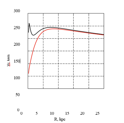
Figure 1: Rotation curve of the Galaxy with an axisymmetric potential without a bar (black line) and a non-axisymmetric potential including a bar (red line).

A cylindrical coordinate system (R, ψ, Z) with the origin of coordinates at the center of the Galaxy is used here. In a rectangular coordinate system (X, Y, Z) with the origin at the center of the Galaxy, the distance to the star (spherical radius) will be equal to r2 = X2 + Y 2 + Z2 = R2 + Z2, while the X axis is directed from the Sun to the galactic center, the Y axis is perpendicular to the axis in the direction of rotation of the Galaxy, and the Z axis is perpendicular to the galactic plane (X, Y ) towards the north galactic pole. The gravitational potential is expressed in units of 100 km2 s−2, distances are in kpc, masses are in units of galactic mass, Mgal = 2.325 × 107M⊙, corresponding to the gravitational constant of G = 1.

Axisymmetric bulge potentials Φb(r(R, Z)) and disk Φd(r(R, Z)) are presented in the form proposed in [14]:

where Mb and Md are the masses of components; and bb, ad, and bd are the scale parameters of components in units of kpc. The halo component (NFW) is presented according to [15]:

Φ (r) = −Mh ln 1 + r!              (4)

r               ah

where Mh is the weight, and ah is the scale parameter. In Table 1, the values of the parameters of the adopted model of the galactic potential are shown.

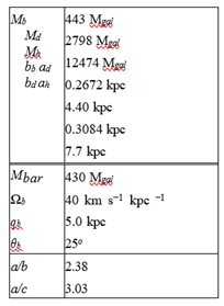
Table 1: Values of the parameters of the galactic potential model, Mgal = 2.325 × 107M⊙

The triaxial ellipsoid model was chosen as the central bar potential [6]: Φbar

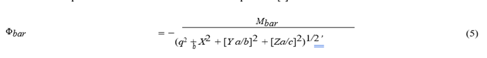
where X = R cos ϑ, Y = R sin ϑ, a, b, c are three semi-axles of the bar, qb is the scale parameter of the bar (length of the largest semi-axis of the bar); ϑ = θ − Ωbt − θb, tg(θ) = Y/X, Ωb is the circular velocity of the bar, t is the integration time, and θb is the orientation angle of the bar relative to the galactic axes X, Y that is measured from the line connecting the Sun and the center of the Galaxy (axis X) to the major axis of the bar in the direction of rotation of the Galaxy. Based on information in the literature, in particular in [7], the following were used as bar parameters: Mbar = 430Mgal, Ωb = 40 km s−1 kpc −1, qb = 5 kpc, and θb = 25o. The accepted bar parameters are listed in 

Table 1. To integrate the equations of motion, we used Runge–Kutta algorithm of the fourth order.

The value of the peculiar velocity of the Sun relative to the local standard of rest was taken to be equal to (u⊙, v⊙, w⊙) = (11.1, 12.2, 7.3) ± (0.7, 0.5, 0.4) km s−1 according to [16]. The elevation of the Sun above the plane of the Galaxy is taken to be 16 pc in accordance with [17].

For comparison, the obtained model rotation curves: an axisymmetric potential (black line) and a potential with a bar (red line) are shown in Fig. 1.

 2 Data

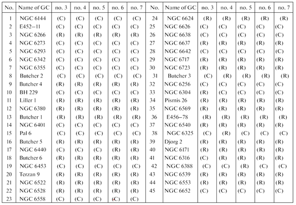
The data on the proper motions of GCs are taken from a new catalogue [4] compiled based on observations of Gaia EDR3. The average values of distances to globular clusters are taken from [5]. The GCs catalogue [18] at our disposal contains 152 objects. Globular clusters from this set belonging to the bulge/bar region were selected in accordance with a purely geometric criterion considered in [19] and also used by us in [20]. It is very simple and consists of selecting GCs whose apocentric distance of orbits does not exceed the bulge radius, which is usually taken to be 3.5 kpc. Orbits were calculated in an axisymmetric potential. The full list of 45 objects in our sample is presented in Table 2, which the results of the analysis of the orbital chaoticity/regularity of GCs (the first column gives the ordinal number of the GCs, the second column gives the name of the GCs) are shown.

We recall the main provisions of the methods considered in this study for determining the nature of orbital dynamics: chaotic or regular. A more detailed description is given in [1–3].

3.1 Poincar´e Sections

The algorithm used to construct the mappings is as follows [21]:

1. We consider the phase space (X, Y, Vx, Vy).

2. We exclude Vy, using the law of conservation of the generalized energy integral (Jacobi integral) and move into space (X, Y, Vx).

3. We define a plane of Y = 0, we will designate the points of intersection with the orbit on the plane (X, Vx). We take only those points, where Vy > 0. If the intersection points of the plane form a continuous smooth line (or several sepa- rated lines), then the motion is considered regular. In the case of chaotic motion, instead of being located on a smooth curve, the points fill a two-dimensional region of phase space, and sometimes the effect of points sticking to the boundaries of islands corresponding to ordered motion occurs [22].

In this paper, we present the Poincar´e sections obtained by us in [1].

3.2 Frequency Method

The method consists of measuring the orbital chaos based on the shift of fundamental frequencies determined over two consecutive time intervals. For each frequency component fi, a parameter called frequency drift is calculated:

where i defines the frequency component in Cartesian coordinates (i.e. lg(∆fx), lg(∆fy), and lg(∆fz))). Then, the largest value of these three frequency drift parameters is at- tributed to the frequency drift parameter lg(∆f ). The higher the value lg(∆f ), the more chaotic the orbit. In order to achieve high accuracy, we took an integration time of 120 billion years, almost an order of magnitude greater than the age of the Universe. In this study, we also used the classification results given in [1].

3.3 Spectral Analysis of Orbits

The spectral analysis of orbits proposed by us in [3] is based on the calculation of the mod- ulus of the discrete Fourier transform (DFT) of uniform time series of radial distances of orbital points from the center of the Galaxy, rn, calculated based on their X, Y, Z galactic coordinates,X(tn), Y (tn), Z(tn) as functions of time: r(tn) =  X(tn)2 + Y (tn)2 + Z(tn)2, where n = 0, ..., N − 1 (N is the length of the row). Thus, the formula for the DFT modulus (amplitude spectrum) of a sequence rn will look like this: 

In this case, the length of the row is selected equal to N = 2α, where α is the positive integer (> 0 ), so that the fast Fourier transform algorithm can be used to calculate the DFT. The required length of the series is achieved by supplementing the real series with zeros. In our case, the length of the actual sequences is 120 000, since we integrate the orbits back 120 billion years with an integration interval of 1 million years. Before calculating the DFT, we first center the coordinate series (i.e., get rid of the constant component), then complement the resulting sequence rn zero readings at n > 120000 until the length of the entire analyzed sequence is reached, N = 262144 = 218. Note that supplementing the initial sequence with zeros is also useful from the point of view of increasing the accuracy of the coordinates of the spectral components. Since the interval between the readings of the sequences in time is equal to δt = 0.001 billion years, then the analyzed frequency range, which is a periodic function, is F = 1/∆t = 1000 Gyr−1. The frequency discrepancy is ∆F = F/N ≈ 0.03815 Gyr−1. Next, for convenience, we will indicate on the graphs not the physical frequencies, but the sample numbers k (or K) of the discrete Fourier transform (2). Transition from k to the physical frequency can be produced by the formula: f = k × ∆F ≈ k × 0.003815. Next, the obtained power spectrum of the GCs orbit is normalized so that the maximal value is equal to unity. The decision on the nature of the orbital dynamics of GCs is determined by calculating the Shannon entropy of the normalized amplitude spectrum r¯k as measures of chaos [23]:

where M is a scale factor that is introduced for the convenience of presenting numerical results. Obviously, the higher the entropy value, the higher the degree of chaos of the orbit. In this case, we analyze both the reference orbits and the shadow ones obtained by perturbing the initial phase point, as accepted in [1–3], as follows: X1 = X0 + X0 × 0.00001, Y1 = Y0 + Y0 × 0.00001, andZ1 = Z0 + Z0 × 0.00001.

3.4 Spectral Analysis of Orbital Coordinates X and Vx

In this work, with the aim of establishing a connection between the Poincar´e sections on the plane (X, Vx) and the spectral characteristics of the orbits, we propose to calculate the modulus of the discrete Fourier transform of uniform time series of coordinates X(tn) and Vx(tn): As an example, the obtained amplitude spectra for two GCs: NGC 6266 and NGC 6355 with regular and chaotic dynamics, respectively, are shown in Fig. 2. As can be seen from the figure and as the analysis of the GC spectra of the entire sample shows, the spectra of the coordinates X and Vx are similar. Therefore, in order to save space, we present below only the spectra of -coordinates in 

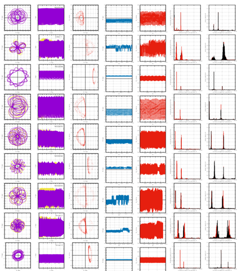
Figure. 3. The same as in the case of the spectral method proposed in [3], regular orbits corre- spond to narrow linear spectra, while chaotic orbits correspond to wide spectra. As will be shown in the next section, this follows, from a comparison of the Poincar´e sections with the results of a spectral analysis, which is the goal of this paper

A graphical representation of the spectral analysis results in comparison with the results obtained previously [1–3] (Poincar´e sections, frequency method, and visual analysis) for the entire sample of 45 GCs is given in Fig. 3, and the results of the classification of orbits into regular (R) and chaotic (C) are given in Table 2 (the first column, as a reminder, shows the serial number of the GCs, while the second column shows the name of the GCs). The proposed method was applied to both reference orbits and shadow orbits. The integration of orbits was carried out, as was already noted above, back 120 billion years. In Fig. 3, it is shown from left to right: (1) projections of orbits onto the plane (X−Y ), (2) radial values of the initial (reference) and perturbed (shadow) orbits depending on time (reference orbits are shown in yellow, shadow orbits are in purple), (3) Poincar´e sections on the plane (X, Vx), (4)X - coordinates of Poincar´e sections, (5)Vx - coordinates of Poincar´e sections, (6) normalized power spectra of X - values of the reference and

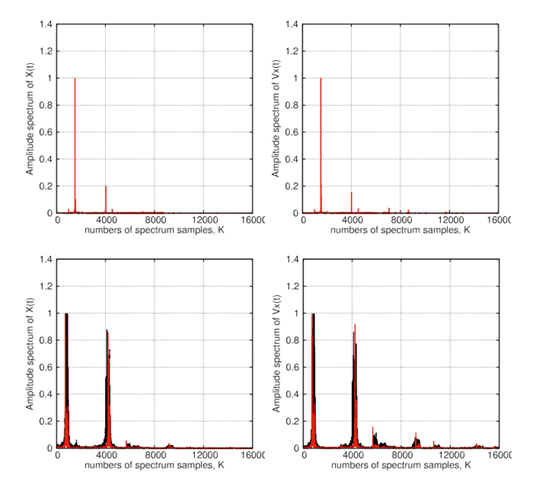
Figure 2: Normalized power spectra of -coordinates (left), -coordinates (right) of the reference and shadow orbits as functions of time that are shown in black and red, respectively. The upper panels refer to GC of NGC 6266 with regular dynamics, and the lower panels refer to GC of NGC 6355 with chaotic dynamics. shadow orbits as functions of time that are shown in black and red, respectively, and (7) illustration of the frequency method (the power spectrum of the first half of the time series is shown in red and the second half is shown in black). The names of the GCs are shown in the second panels from the left. The most obvious illustration of the discrepancy between the reference and shadow phase points are columns 1 and 2 in Fig. 3, which list the reference and shadow orbits for each GC in the order (top to bottom) as they are listed in Table 2. The first column contains X, Y projections of orbits constructed in the rotating bar system over a time interval of [−11, −12] billion years. The second column shows the radial values of the orbit r(t) on the interval of [0, −12] billion years that is comparable to the age of both GCs and the Universe. In these graphs, reference orbits are shown in yellow, and shadow orbits are shown in purple. As can be seen, many objects on the graphs have purple color only. This means that the shadow orbit is almost identical to the reference orbit (yellow lines are covered with purple ones). Such objects include GCs with regular orbits. In the graphs of GCs with chaotic orbits, both purple and yellow lines are visible, which makes it possible to judge qualitatively the degree of chaos of the orbits. In the third column, the Poincar´e sections on the plane (X, Vx) are shown. Dependence of coordinates X and Vx on the counting number are given in the fourth and fifth columns, respectively. The regularity of the distribution of coordinates X and Vx characterizes the regularity of orbital dynamics, and this is reflected in the Poincar´e sections. As in the case of the spectral method proposed in [3], as well as the frequency method, the normalized amplitude spectra of the reference and shadow orbits that are given in the sixth and seventh columns have the character of line spectra for GCs with regular dynamics and broad spectra for GCs with chaotic dynamics. 

The obtained amplitude spectra of coordinates X and Vx show a one-hundred-percent correlation with the nature of the distribution of points on the Poincar´e sections, which is reflected in the sixth and seventh columns of Table 2, which also present the results of the classification of GCs with regular and chaotic orbits from previous studies [1, 3], obtained using: the spectral-entropy method [3] (third column of the table), the frequency method (fourth column) [1], and the visual method (fifth column) [1]. Based on an analysis of the table, a high correlation between the results of GC classification by different methods (not less than 82.5%) is shown. Due to the established connection between Poincar´e sections and the spectral method for the analysis of orbital dynamics instead of Poincar´e sections, the decision-making process for which is characterized by some subjectivity, a more visual method of the spectral analysis can be used. From the fact that the classification by Poincar´e sections completely coincides with the classification by the width of the amplitude spectrum, we have defined two lists. The first list includes 25 globular clusters with regular dynamics (R) (NGC 6266, Terzan 4, Liller 1, NGC 6380, Terzan 1, Terzan 5, NGC 6440, Terzan 6, Terzan 9, NGC 6522, NGC 6528, NGC 6624, NGC 6637, NGC 6717, NGC 6723, Terzan 3, Pismis 26, NGC 6569,NE456–78, NGC 6540, Djorg 2, NGC 6171, NGC 6316, NGC 6539, and NGC 6553) and a second list of 20 globular clusters with chaotic dynamics (C) (NGC 6144, E452–11, NGC 6273, NGC 6293, NGC 6342, NGC 6355, Terzan 2, BH 229, NGC 6401, Pal 6, NGC 6453, NGC 6558, NGC 6626, NGC 6638, NGC 6642, NGC 6256, NGC 6304, NGC 6325, NG 6388, and NGC 6652). Furthermore, from the second list, we consider it appropriate to select GCs with varying degrees of chaos using the entropy measure. For example, we classified GCs NGC 6144, NGC 6273, NGC 6304, NGC 6325, and NGC 6388 as GCs with weakly chaotic dynamics. GCs E452–11, NGC 6355, Terzan 2, BH 229, NGC 6401, Pal 6, NGC 6558, NGC 6638, NGC 6642, and NGC 6652 exhibit strong chaos.

The following main results were obtained: 4.1 A direct, 100% connection has been established between the Poincar´e sections of regular and chaotic orbits and the spectral characteristics of the orbits. The wider the spectrum, the higher the entropy and the more chaotic the orbital character is shown by the Poincar´e section. Thus, for the analysis of orbital dynamics, instead of Poincar´e sections, the classification by which is somewhat subjective, a more visual method of spectral analysis of orbits can be used. 4.2 Based on the established relationship between the Poincar´e sections and the spectral characteristics of the orbits, of 45 GCs in the central region of the Galaxy with a radius of 3.5 kpc, a list of 25 globular clusters with regular dynamics (R) was determined:

NGC6266, Terzan4, Liller1, NGC6380, Terzan1, Terzan5, NGC6440, Terzan6, Terzan9, NGC6522, NGC6528, NGC6624, NGC6637, NGC6717, NGC6723, Terzan3, Pismi26, NGC6569, E456-78, NGC6540, Djorg2, NGC6171, NGC6316, NGC6539, and NGC6553 and a list of 20 globular clusters with chaotic dynamics (C): NGC6144, E452-11, NGC6273, NGC6293, NGC6342, NGC6355, Terzan2, BH229, NGC6401, Pal6, NGC6453, NGC6558, NGC6626, NGC6638, NGC6642, NGC6256, NGC6304, NGC6325, NGC6388, and NGC6652. 4.3 From the list of GCs with chaotic dynamics, one can identify GCs with varying degrees of orbital chaos based on a comparison of the entropy measure. We classified GCs NGC6144, NGC6273, NGC6304, NGC6325, and NGC6388 as weakly chaotic. GCs E452–11, NGC 6355, Terzan 2, BH 229, NGC 6401, Pal 6, NGC 6558, NGC 6638, NGC 6642, and NGC 6652 show strong chaos.

References

- A. T. Bajkova, A. A. Smirnov, and V. V. Bobylev, Publ.
View at Publisher | View at Google Scholar - (2024); arXiv: 2406.15590 [astro-ph.GA].
View at Publisher | View at Google Scholar - A. T. Bajkova, A. A. Smirnov, and V. V. Bobylev, Publ. (2024); arXiv: 2412.02426 [astro-ph.GA].
View at Publisher | View at Google Scholar - A. T. Bajkova, A. A. Smirnov, and V. V. Bobylev, Publ. (2025).
View at Publisher | View at Google Scholar - E. Vasiliev and H. Baumgardt, Mon. Not. R. Astron. Soc. 505, 5978 (2021); arXiv: 2102.09568 [astro-ph. GA].
View at Publisher | View at Google Scholar - H. Baumgardt and E. Vasiliev. Mon. Not. R. Astron. Soc. 505, 5957 (2021); arXiv: 2105.09526 [astro-ph. GA].
View at Publisher | View at Google Scholar - J. Palous, B. Jungwiert, and J. Kopecky, Astron. Astrophys. 274, 189 (1993).
View at Publisher | View at Google Scholar - J. L. Sanders, L. Smith, N. W. Evans, and P. Lucas, Mon. Not. R. Astron. Soc. 487, 5188 (2019); arXiv: 1903.02008 [astro-ph.GA].
View at Publisher | View at Google Scholar - R. E. G. Machado and T. Manos, Mon. Not. R. Astron. Soc. 458, 3578 (2016); arXiv: 1603.02294 [astro-ph. GA].
View at Publisher | View at Google Scholar - N. Nieuwmunster, M. Schultheis, M. Sormani, F. Fragkoudi, F. Nogueras-Lara, R. Schodel, and P. McMillan, arXiv: 2403.00761 [astro-ph.GA] (2024).
View at Publisher | View at Google Scholar - M. Valluri, V. P. Debattista, T. Quinn, and B. Moore, Mon. Not. R. Astron. Soc. 403, 525 (2010); arXiv: 0906.4784 [astro-ph.CO].
View at Publisher | View at Google Scholar - J. Laskar, Celest. Mech. Dyn. Astron. 56, 191 (1993).
View at Publisher | View at Google Scholar - M. Valluri and D. Merritt, Astrophys. J. 506, 686 (1998).
View at Publisher | View at Google Scholar - E. Vasiliev, Mon. Not. R. Astron. Soc. 434, 3174 (2013).
View at Publisher | View at Google Scholar - M. Miyamoto and R. Nagai, Publ. Astron. Soc. Jpn. 27, 533 (1975).
View at Publisher | View at Google Scholar - J. F. Navarro, C. S. Frenk, and S. D. M. White, Astrophys. J. 490, 493 (1997).
View at Publisher | View at Google Scholar - R. Sch¨onrich, J. Binney, and W. Dehnen, Mon. Not. R. Astron. Soc. 403, 1829 (2010).
View at Publisher | View at Google Scholar - V. V. Bobylev and A. T. Bajkova, Astron. Lett. 42, 1 (2016).
View at Publisher | View at Google Scholar - A. T. Bajkova and V. V. Bobylev, Publ. Pulkovo Observ. 227, 1 (2022); arXiv: 2212.00739 [astro-ph.GA].
View at Publisher | View at Google Scholar - D. Massari, H. H. Koppelman, and A. Helmi, Astron. Astrophys. 630, L4 (2019).
View at Publisher | View at Google Scholar - A. T. Bajkova, G. Carraro, V. I. Korchagin, N. O. Budanova, and V. V. Bobylev, Astrophys. J. 895, 69 (2020).
View at Publisher | View at Google Scholar - C. D. Murray and S. F. Dermott, Solar System Dynamics (Cambridge Univ. Press, Cambridge, 2012).
View at Publisher | View at Google Scholar - A. Morbidelli, Modern Celestial Mechanics: Aspects of Solar System Dynamics
View at Publisher | View at Google Scholar - (Taylor and Francis, London, 2002).
View at Publisher | View at Google Scholar - O. V. Chumak, Entropy and Fractals in Data Analysis (Inst.
View at Publisher | View at Google Scholar